How to run simulations

Workflow

The essential workflow to run simulations with Quokka3 consists of 3 separate steps:

1. Define your simulation input parameters in a settingsfile within a text-editor of your choice (Notepad++ is a good choice). See finding the right parameter for the ways to look up the available parameters.
2. Start the simulation and manage cloud simulations. For larger cloud simulations, the recommended way is to start the simulation, disconnect, and retrieve the results once finished.
3. Post-process the results via the GUI’s basic plotting functionality, or by processing the output files yourself.

There are three ways to drive Quokka3, all using the same settingsfiles and the same cloud account:

• the GUI: start and control simulations, inspect the geometry in the 3D view and the results in quick plots.
• the command line (Quokka3_cmd): scripted simulation control.
• MCP: let your own AI assistant (e.g. Claude Code, Cursor or VS Code) look up settings, validate settingsfiles, and run and manage cloud simulations for you. Quokka3 provides the tools, the knowledge and the compute; the AI is yours.

Whenever you are stuck, the quickest help is Ask Quokka, the chat assistant at the bottom right of every page on www.quokka3.com (also at the end of this page). It knows the Quokka3 manuals and solar cell modelling, is free to use, and gives licensed users a higher usage limit when signed in with their cloud account. It is the only AI feature operated by us: the GUI, the command line, the simulation core and the cloud service contain no AI.

The core of Quokka3, which performs the actual simulations, comes in two ways:

• a restricted free version, which is included as a standalone executable and runs locally on your computer.
• the full version, which exclusively runs as a cloud service controlled via the Quokka3 client, and consequently requires an internet connection and a user account.

The way of controlling simulations is (almost) identical regardless of whether you use the included free version or the cloud service.

The free version is meant for learning and for small simulations (see the licensing page for the terms). It is restricted to:

• 1D and 2D solution domains of up to 1 cm lateral size: no 3D domains, which excludes busbar-enhanced unit cells, full-cell and multi-domain simulations
• silicon as bulk material, with a homogeneous background doping (no bulk doping profiles)
• lumped skins on the front and rear side only: no detailed (multiscale) skins, no skin solver, no layers within a skin, no vertical skin resistivity
• single-junction, contacted devices with ohmic contacts: no tandem / multi-junction cells, no equivalent-circuit bulk model, no finite-differences metal model
• small meshes (about 10k elements for a semiconductor device, 50k for a purely resistive one), sweeps of up to 100 points, and no optimizer

If a settingsfile exceeds these limits, the free core stops with a message naming the restriction.

Note that for the cloud, it sometimes might take up to a couple of minutes for the simulation to start, because cloud servers are started on demand. Only very rarely this delay is significant compared to the overall simulation time.

If a connected cloud simulation finishes, or a finished cloud simulation is opened or downloaded, the results are automatically downloaded and deleted from the cloud. Results that are never downloaded are deleted after 120 days. Only some anonymous metadata like simulation time, memory usage etc. are kept for statistical and service-improvement purposes.

System requirements

Quokka3 runs on Windows (64-bit) and on macOS (Apple silicon). Installation is required both for free and full-version usage. As the included standalone free core executable allows only small simulations, and large simulations are exclusively performed in the cloud, Quokka3 doesn’t require highly performant computer hardware for simulations. It should work on any reasonably up-to-date computer.

The 3D view of the GUI uses OpenGL (version 3.2 or newer, which any current graphics driver provides). If the 3D view stays empty or shows artefacts, updating the graphics driver usually fixes it.

To use the full version, the computer must have internet connection to access the cloud service. Connection is made over the standard https protocol on its default port 443, making it indifferent to browsing websites. However, sometimes internet access for newly installed software is blocked by company firewall settings, in which case you should check your firewall / malware settings and add an exception. Quokka3 also supports the use of a proxy server, see the cloud options.

Installation

First, download the current version of Quokka3:

• Windows: run the installer (which needs administrator rights for the default location C:\Program Files\Quokka3), or extract the zip archive into a folder of your choice, which works without administrator rights.
• macOS: open the .dmg and drag Quokka3 into your Applications folder. The app is signed and notarized.

Quokka3 consists of the following files (Windows: in the bin folder of the installation, or the extracted zip folder; macOS: inside the Quokka3.app bundle under Contents/Resources):

• Quokka3.exe / Quokka3.app: the main Quokka3 application, starts the GUI
• q3core.exe / q3core: the free core executable for performing local offline simulations; it is restricted in functionality, the full version can only be accessed via the cloud service
• Quokka3_cmd.exe / Quokka3_cmd: allows simulation control via the command-line
• q3_optical_data.h5: a database of optical material properties used by the core
• config.ini: created on first start in your application data folder (Windows: %APPDATA%\Quokka3\config.ini, macOS: ~/.Quokka3/config.ini); it contains the client configuration, you do normally not need to open that file yourself

Compute capacity

Cloud compute time is unlimited on every full license. There is no CPU-hour quota, no metering and no throttling — you can keep the cloud busy 24/7 if your work calls for it.

What your license sizes is capacity: the CPUs and RAM that can be running at the same time. The figures are stated in your license quote.

Capacity is enforced at two levels — your own limit and the license total — and both are checked when a simulation is dispatched. If a simulation does not fit right now, because your own runs or other users’ runs are occupying the capacity, it simply waits in the queue and starts as soon as room frees up. It is not refused and nothing is lost. Only a simulation larger than your limit could ever allow is rejected at submission, immediately and with a clear message.

Capacity pools within a license. The totals belong to the license, not to individual people. License admins set each user’s CPU and RAM limits in the manage dialog, up to the license total — including giving most of the capacity to a single power user. Because every additional seat — one user account, with its own CPUs and RAM — adds to the license total, holding an additional seat purely for capacity is a supported way to increase one person’s parallel compute.

In practice:

• For each cloud simulation you choose the number of CPUs (up to 8, and never more than your own CPU limit). The RAM demand is predicted by the client from the mesh size before anything is uploaded. A simulation that can never fit your limits, or that exceeds what a single cloud server can run (8 CPUs, 15 GB RAM), is refused immediately with a message; anything else is accepted and starts as soon as capacity is free.
• Every user can see their own usage via the details button in the Simulation Control panel: the CPUs and RAM currently in use against the personal and the license limits.
• License admins distribute the capacity among the users of the license in the manage dialog.

GUI

The purpose of the GUI is to conveniently control simulations and provide some basic results plotting functionality. It is not for defining the actual simulation parameters, which is done in the settingsfile. The plotting functionality provides a quick way to inspect main results, but it is not scoped to be a powerful generic post-processor. If you want to plot the results in a particular way of your liking, you need to read the results data from the results files and create the plots with your own tools.

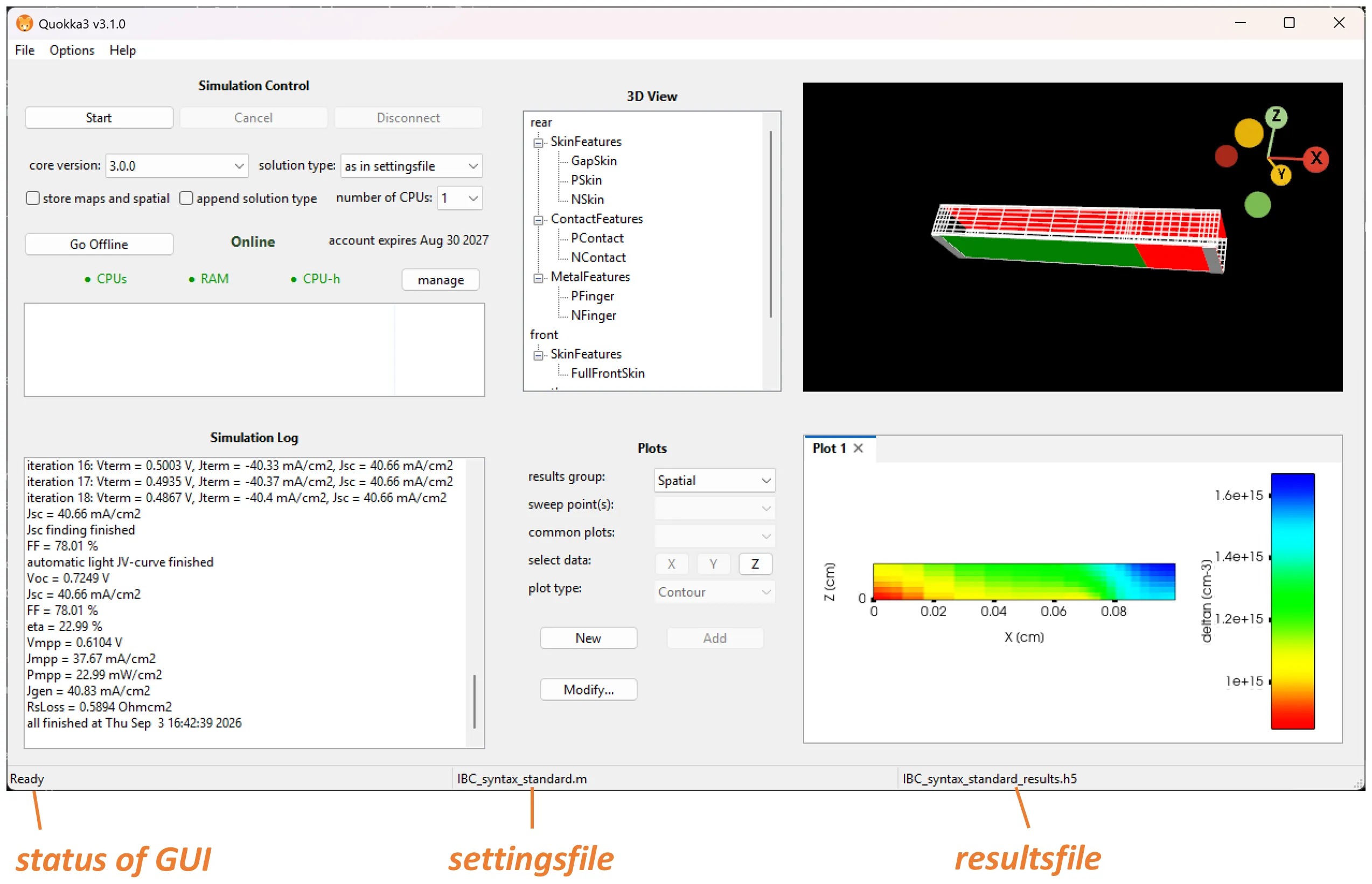
The GUI features a File, Options and Help menu at the top, and a bottom section with the current status of the GUI, the currently loaded settingsfile and resultsfile. The main area consists of 4 panels:

• Simulation Control: Let’s you start and cancel local or cloud simulations, go online, show a list of current cloud simulations, and some other simulations controls.
• Simulation Log: displays the mesh size and warnings when a settingsfile is loaded, live output during a running simulation, or the log of a finished simulation when downloaded from the cloud.
• 3D View: displays the geometric features and numerical 3D mesh of the last loaded settingsfile or resultsfile in a mouse-interactive view. Right-clicking on any item in the tree list will give some options to toggle visibility and highlighting that geometric item. You can double-click in the 3D view area to get a full-screen view.
• Plots: After a finished simulation, or after opening a resultsfile, you can create various kinds of plots in this panel. First select a results group, and then proceed downwards with data selection (an exclamation mark ”!” means you have to select data by clicking on that button), until the “New” or “Add” button let’s you create a new plot or append the data to the current plot. Clicking “Modify” let’s you change the current plot, e.g. axis limits and linear / log scale.

File menu

In the file menu you can open a settingsfile or resultsfile, and reload the current settingsfile (F5) after editing it. Opening or reloading a settingsfile meshes the geometry locally, shows it in the 3D view, and prints the mesh size, warnings and any unused settings to the Simulation Log. It is good practice to always check the geometry and mesh size this way before starting simulations; it takes only seconds, and works also when connected to the cloud.

The “Export” function allows you to:

• Export Excel resultsfile: writes an Excel file for the currently opened resultsfile, see results files; for sweeps you are asked how many sweep points to include.
• Export a generic settingsfile: this is useful if your settingsfile is created in a simplified syntax and you want to have the exact same settings in the generic syntax in order to make some modifications not possible within the simplified syntax.
• Export 3D view: exports the current 3D view with various image and 3D formats available.
• Export current plot: let’s you export the current plot’s data as a csv file, or as various image formats.

Options menu

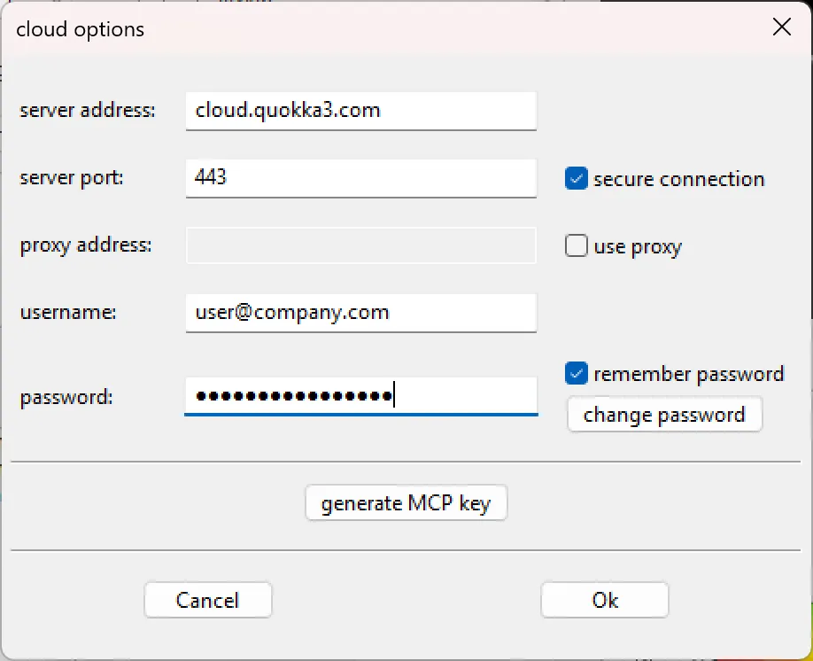
Via Options → Cloud … the cloud options are accessible, which are required to enter if you want to access the full version via the cloud service. Enter the username and password as provided during the licensing.

If your computer uses a proxy server to connect to the internet, then activate “use proxy” and enter the server and port in the format “server:port” in the proxy address field.

The default connection to the cloud server “cloud.quokka3.com” is done via a SSL secured connection on port 443, which is the typical way for end-to-end encrypted secure internet data transfer. It is also possible to connect to the cloud server without secure connection on port 80 by unchecking “secure connection”, which may be useful for debugging purposes, or if encrypted internet connection is not strictly required.

When checking “remember password”, Quokka3 securely stores the password in the Windows Credential Manager or the macOS Keychain on your local computer, so you don’t need to re-enter it every time you connect to the cloud.

The dialog also has two buttons: change password for your own account, and generate MCP key to connect your AI assistant, see MCP.

Help menu

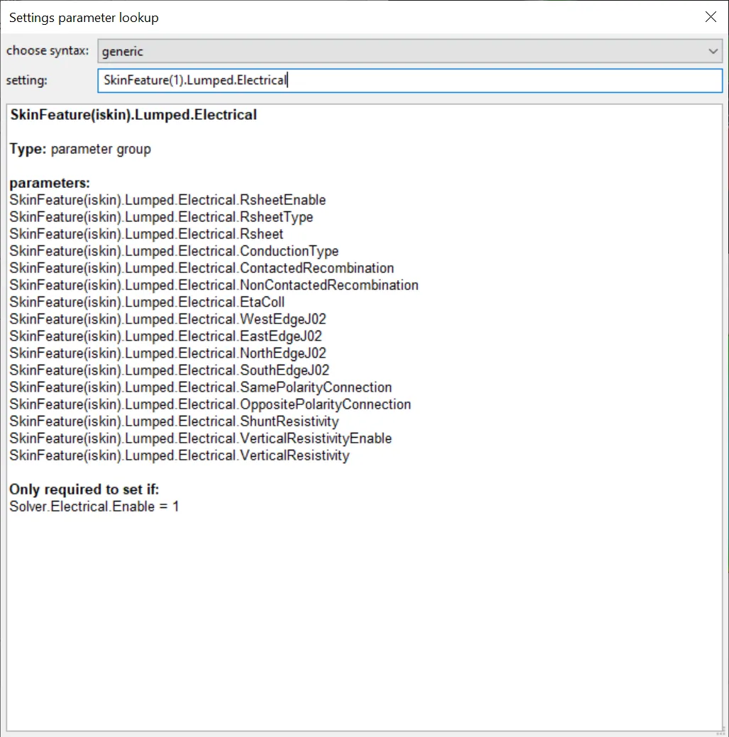
In the help menu you find the settings lookup, which lists all parameters available for a settingsfile of the installed version. First select a syntax for which you’d like to lookup a settings parameter. You will then already see a list of all available settings groups within that syntax. You can then enter any group, subgroup, or parameter in the text field, or copy-paste it from a settingsfile. After pressing “Enter” you will get a description and other information like dependencies which need to be fulfilled in order for that parameter to be applicable.

The settings lookup is one of several ways to find a parameter; the online Settings Reference and Ask Quokka are usually the faster ones, see finding the right parameter.

Simulation Control

Here you start, cancel and disconnect simulations, and connect to the cloud (“Go Online”; the button then reads “Go Offline”, and the panel shows your account’s expiry date). When offline, “Start” runs the free local core; when online, it starts a cloud simulation. The controls are:

• core version: the core version used in the cloud; you can select a previous version, e.g. if the current one introduced a problem for your case.
• solution type: overrides the solution type in the settingsfile, to quickly simulate a variety of characteristics once your device properties are defined. If you enable append solution type, the name of the resultsfile will contain the solution type, which is useful to not overwrite results of the same settings just with a different solution type.
• store maps and spatial: identical to setting SaveSpatial = 1; and SaveMaps = 1; in the settingsfile. It forces Quokka3 to store spatial and map results in the resultsfile. If not checked, this data will not be stored for larger simulations to save on filesize.
• number of CPUs: the number of CPUs for a cloud simulation, up to 8 and limited by your personal CPU limit. Several CPUs speed up sweeps, whose sweep points are then solved simultaneously; a single simulation point always runs on one CPU, so choose at most as many CPUs as sweep points.

Once online, the lower box lists your cloud simulations with their current status. You may disconnect a running simulation and start more simulations until the license limits or your personal limits for CPU and RAM have been reached; disconnecting a simulation does not interrupt it. Right-click a simulation to reconnect to or abort a running one, to download or delete a finished one, or to show the log of a failed one. Downloaded results are deleted from the cloud, see workflow.

The three indicators CPUs, RAM and CPU-h show your usage at a glance: green while you have room, orange from 75 % of your personal limit, red when the limit is reached (a further simulation would then wait for capacity); CPU-h is informational only, as compute time is unlimited. The details button next to them shows your current cloud usage in numbers. For license admins it is named manage and additionally opens the cloud management.

Cloud management

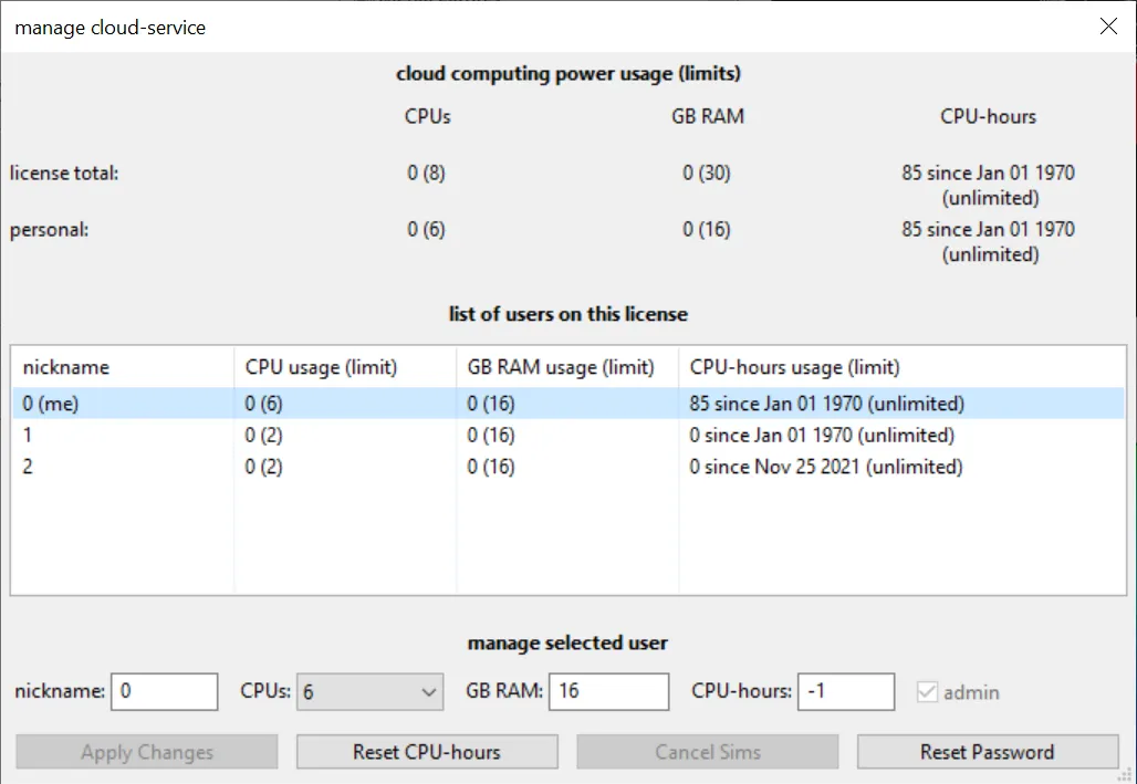
When you click the “manage” button as a license admin, you will see the license’s current usage and a list of the users on that license with their CPU and RAM limits. Select a user to manage it:

• set the user’s share of the license’s CPU and RAM capacity and its nickname, or make the user an admin as well by checking “admin”, then click “Apply Changes”;
• “Reset Password” sets a new password, e.g. in case of a forgotten password (note this invalidates that user’s MCP key, if one exists);
• “Cancel Sims” cancels all running simulations of that user, e.g. if a user is accidentally using up all CPUs or RAM.

Note that the actual usernames are not shown in the list, as they are only stored encrypted in the cloud for data security. You rather see the “nicknames” of the users, which default to the initials or first letters of the login name, and which you are free to set to whatever you like in order to identify the users.

The addition of new users or removal of existing users can currently not be performed by the license admin. Please get in contact if you wish to add or remove user accounts on your license.

Updates

The GUI checks for updates each time you connect to the cloud. If a new version is available, a popup window shows its changelog, with the options to update now or later. Updating works completely automated: the new files are downloaded and copied over the installation (on Windows, the previous files are kept as previous_* until the next update), and Quokka3 is restarted (on macOS, start it again yourself if it does not reappear). Alternatively, download and install the latest version yourself.

Updating is strongly recommended: an outdated version is refused by the cloud service, both the GUI and the command line will tell you to update.

Command-line

For scripted simulation control a command-line interface is provided via Quokka3_cmd.exe (Windows, located next to Quokka3.exe) or Quokka3_cmd (macOS, located inside the app bundle at /Applications/Quokka3.app/Contents/Resources/Quokka3_cmd). The basic format to use it is

>Quokka3_cmd.exe [COMMAND] [PARAM1] [PARAM2]

The return code is -1 on error and 0 for success. Only the command START_LOCAL uses the local free version, all other commands control cloud simulations. They use the cloud options as set in the GUI; if no password is stored there, the command line asks for it on standard input, so it can also be piped in from a script. Like the GUI, the command line refuses cloud commands when the installed version is outdated for the cloud service.

The available commands are

START_LOCAL <settingsfile>
START_WAIT <settingsfile> [numCPU] [timeoutHours]
START_DISCONNECT <settingsfile> [numCPU]
LIST
STOP <simID>
GET_LOG <simID>
DOWNLOAD_RESULTS <simID>
DELETE <simID>

All commands taking a SIMULATION ID work on the raw id, whichever Quokka3 version created the simulation.

START_LOCAL

Starts a local simulation, i.e. using the free Quokka3-core executable. PARAM1 is the settingsfile, PARAM2 is not used. Example:

>Quokka3_cmd.exe START_LOCAL "C:\my folder with spaces\mysettingsfile.m"

START_WAIT

Starts a cloud simulation, continuously displays the log, downloads results and deletes the simulation from the cloud. PARAM1 is the settingsfile, PARAM2 is the number of cores to be used, and the optional PARAM3 is a timeout in hours (default 24). Example:

>Quokka3_cmd.exe START_WAIT "C:\my folder with spaces\mysettingsfile.m" 2 6

When the timeout expires the command returns, but the simulation keeps running in the cloud — it is not stopped. The printed hints tell you how to reconnect to it or to stop it by its SIMULATION ID.

Pressing Ctrl-C stops the cloud simulation cleanly rather than just abandoning the console: the stop request is sent, the simulation is aborted server-side, and the compute stops.

START_DISCONNECT

Starts a cloud simulation and immediately returns. PARAM1 is the settingsfile, PARAM2 is the number of cores to be used. The last output message is the SIMULATION ID, which is required for the GET_LOG and DOWNLOAD_RESULTS commands. Example:

>Quokka3_cmd.exe START_DISCONNECT "C:\my folder with spaces\mysettingsfile.m" 2

LIST

Lists all your cloud simulations, across every Quokka3 version, as a tab-separated table with a header row — readable, and easy to grep or parse in a script. Takes no parameters. The columns are

ID  NAME  STATUS  VERSION  CPU  RAM_GB  DURATION_S  FILESIZE_MB  LOADABLE

followed by a count line. LOADABLE says whether this client version would select that simulation’s version for opening or submitting; it does not restrict STOP, DELETE, GET_LOG or DOWNLOAD_RESULTS, which all work on the raw id regardless of version. Example:

>Quokka3_cmd.exe LIST

GET_LOG

Retrieves and prints the log of a cloud simulation, whether it is still running or finished. PARAM1 is the SIMULATION ID, PARAM2 is not used. Example:

>Quokka3_cmd.exe GET_LOG 1495811542680

DOWNLOAD_RESULTS

Downloads results of a finished cloud simulation and deletes it from the cloud; for a simulation that is still running it returns with an error message. PARAM1 is the SIMULATION ID, PARAM2 is not used. Example:

>Quokka3_cmd.exe DOWNLOAD_RESULTS 1495811542680

STOP

Stops a running cloud simulation. PARAM1 is the SIMULATION ID, PARAM2 is not used. The simulation is aborted server-side and the compute stops; the simulation itself stays in your list until you delete it. Example:

>Quokka3_cmd.exe STOP 1495811542680

DELETE

Deletes a cloud simulation and its result files. PARAM1 is the SIMULATION ID, PARAM2 is not used. Deletion is permanent. Example:

>Quokka3_cmd.exe DELETE 1495811542680

MCP

Besides the GUI and the command line, Quokka3 can be driven by an AI assistant via the Model Context Protocol (MCP) — the open standard by which AI applications such as Claude Code, Claude Desktop, Cursor or VS Code connect to external tools. Once connected, your assistant can search the curated Quokka3 knowledge base, look up settingsfile parameters, validate settingsfiles against the authoritative schema of the current release, and start and manage cloud simulations on your account.

The MCP integration is available to licensed users and requires a personal MCP key. You bring your own AI: Quokka3 provides the tools, compute and knowledge, while your assistant provides the reasoning (and its own inference cost). If you just have a question about Quokka3, Ask Quokka on www.quokka3.com is the quicker route; MCP is for letting your assistant do the work.

Generating your MCP key

In the GUI, open Options → Cloud … and click generate MCP key, then re-enter your password. The key is displayed once, together with its expiry date and a copy-to-clipboard button — store it in your MCP client configuration (see below), not anywhere public. There is exactly one active key per user: generating a new key revokes the previous one, and a password change (your own, or forced by an admin) also invalidates it. In both cases simply generate a new key. Use the same key in every MCP client you run (a second computer, a second assistant): generating another key for the other machine would revoke the first. The key’s expiry is fixed when it is generated (at most one year, never beyond your license), so after a license renewal generate a new key to extend it.

If you cannot use the GUI, a key can also be generated directly (note that username and password may end up in your shell history — prefer the GUI dialog):

curl -X POST "https://cloud.quokka3.com/QuokkaRest/v2/auth/mcp/key" --data-urlencode "username=USERNAME" --data-urlencode "password=PASSWORD"

The JSON response contains the key and its expiry date.

Connecting your AI assistant

The Quokka3 MCP server is a remote server — there is nothing to install locally. Add it to any MCP-capable host application, using your MCP key as the authorization token. Example configuration (Claude Code / Claude Desktop style; other hosts need the same two pieces of information):

"quokka3": {
  "type": "http",
  "url": "https://mcp.quokka3.com/mcp",
  "headers": { "Authorization": "Bearer YOUR-MCP-KEY" }
}

What your assistant can do

Tool	Purpose
search_knowledge_base	grounded answers from the curated Quokka3 knowledge base — model choice, gotchas, version specifics
lookup_setting	exact parameter reference: type, unit, bounds, options, default, dependencies
validate_settings_file	checks a settingsfile against the release schema and the authoritative server-side checker
search_manual, list_examples / get_example	the manuals and the worked examples
run_simulation, get_simulation_status, get_simulation_logs, stop_simulation, delete_simulation, list_simulations	the cloud-simulation lifecycle, equivalent to the command-line workflow
get_contingents, list_versions	your current compute capacity and usage; available Quokka3 versions
download_results	download links for the results of a finished simulation

Compute usage via MCP

Simulations started through MCP run on your account and draw on the same compute capacity as GUI or command-line simulations — an agent submitting many simulations queues behind your CPU and RAM limits like any other usage. Compute time itself is unlimited, so an assistant cannot exhaust an allowance; it can only wait for capacity. Where a submission is refused, the assistant receives the same explanatory message the GUI shows.

Before anything is uploaded, every MCP submission is prepared exactly as the GUI prepares its own: the geometry is meshed, the required RAM is predicted, and the settingsfile together with all referenced input files travels as a single bundle. Simulations submitted by an assistant are therefore sized and scheduled identically to GUI submissions, and a run larger than your capacity limits is refused before it starts — it costs nothing.

Settingsfile

Structure

All input parameters for the device properties and its characteristics to be simulated are defined in a settingsfile. It is a plain ASCII text file which can be edited by any text editor of your choice. While any extension is supported (e.g. *.txt), it is recommended to use *.m as the extension. It is noted however that the settingsfile is NOT interpreted as a Matlab-script, in particular no variables or mathematical expressions are supported. The *.m extension is solely useful to enable syntax highlighting in text-editors (e.g. Notepad++), as the settings syntax is derived from the Matlab syntax (mainly commenting via ”%” and vector definition).

The settings consist of a list of assignments in the following exemplary form:

group.subgroup.parameter = value [unit]; % comment

There are four different types of values (no other types like variables or expressions are supported):

• switch: to enable or disable something by setting it to 1 or 0 respectively
• scalar: a single numeric value excluding any unit, which can be set in common formats (e.g. 110, 1.1e2 or 1.1E+02); you can add a unit, e.g. 15 fA/cm2, otherwise the default unit is used; for available units of a particular parameter see finding the right parameter
• string or option: a string value needs to be given in ‘single quotes’
• vector: a series of scalar values which can be defined in various ways, also with unit support

Some settings require the input of two-column tabulated (XY) data points, e.g. for the generation profile. There is a common way to define such XY input data, including via loading it from a file.

Quokka3 supports various syntaxes for providing a generic way of defining the simulation setup (generic syntax), as well as simplified ways for various common simulation tasks (simplified syntaxes). With the considerably large functionality of Quokka3, the generic syntax unavoidably results in longish parameter names from nested groups. For an easier start simplified syntaxes are recommended, mainly simplifying geometry definitions, which as a compromise address only a subset of Quokka3 functionality.

The settings are organized into various levels of groups separated by a dot; only a few top-level settings such as Syntax, SaveSpatial and SaveMaps stand alone, see the common settings in the Settings Reference. In the following tables, the parameters need to be preceded by the respective name of the group. Default settings are marked with an Asterisk* and are not required to be given.

Finding the right parameter

There are four ways to find out which parameters exist, what they mean, and which values, units and dependencies they have:

1. The online Settings Reference: the complete parameter list of the current version, one section per syntax, searchable with your browser.
2. Ask Quokka, the chat assistant on every page of www.quokka3.com (also at the end of this page): ask in plain language, e.g. “how do I define a lifetime curve from a file?”, and get the matching parameters together with modelling advice. This is usually the fastest way.
3. The settings lookup in the GUI’s Help menu, which reflects exactly the installed version.
4. Via MCP, your own AI assistant can look up parameters and validate a complete settingsfile for you.

Sweep

A sweep varies input parameters for a series of defined values. It supports two independent sweep groups A and B, within each multiple parameters can be varied at the same time. Within each group, the number of sweep values must be equal for all parameters. That means that (up to) a 2-dimensional sweep can be defined, where each dimension can consist of multiple simultaneously varied parameters. If a higher dimensional sweep it desired it is up to the user to linearize it into a 2- or 1-dimensional sweep.

There are some advantages of doing the sweep within Quokka3:

• gives a single results file summarizing all sweep results
• plotting functionality of GUI has the capability of quickly plotting main results as a function of the sweep parameters
• can be run in parallel mode to solve sweep points simultaneously
• Performance is better in certain scenarios, as Quokka3 can re-use some results from previous sweep-points for a faster simulation

Sweep settings group:

parameter	(recommended) value range	description
.Enable	1 / 0	enables / disables the sweep functionality
.NGroups	1 / 2	number if independent sweep groups; 1 means group A only, 2 means group A and B
.GroupA(ia).Parameter	’parameter name’	can be any switch, scalar, string or option parameter, e.g. it is also possible to sweep filenames; multiple, consecutively indexed parameters can be defined
.GroupA(ia).Values	vector	vector of values; the same unit as for the respective parameter applied; all vector values within a group must have the same length
.GroupB(ib).Parameter	’parameter name’	same as for GroupA
.GroupB(ib).Values	vector	same as for GroupA

As an example, the sweep settings

Sweep.Enable = 1; % enable sweep
Sweep.NGroups = 2;
Sweep.GroupA(1).Parameter = 'SkinFeature(1).Lumped.Electrical.Rsheet';
Sweep.GroupA(1).Values = [70 100 150];
Sweep.GroupA(2).Parameter = 'SkinFeature(1).Lumped.Electrical.J0'; % dependent parameter: higher Rsheet means lower J0
Sweep.GroupA(2).Values = [150 100 70]*1e-15;
Sweep.GroupB(1).Parameter = 'Bulk.Electrical.Recombination.LifetimeCurve.File'; % independent parameter
Sweep.GroupB(1).Values = ['file_1.csv' 'file_2.csv'];

will simulate the following 6 sweep points (shown in linearized form):

#	ia	ib	Rsheet	J0	File
1	1	1	70	150e-15	’file_1.csv’
2	1	2	70	150e-15	’file_2.csv’
3	2	1	100	100e-15	’file_1.csv’
4	2	2	100	100e-15	’file_2.csv’
5	3	1	150	70e-15	’file_1.csv’
6	3	2	150	70e-15	’file_2.csv’

XY input

XY-input settings group:

parameter	(recommended) value range	description
.Type	’const’, ‘XY’, ‘file’	how to define XY values; ‘const’: constant Y value for any X value; ‘XY’: definition of X vector and Y vector; ‘file’ read XY values from a 2-column ASCII file
.Const		constant Y value; unit as given in the parameter description
.X	vector	vector of X values; unit as given in the parameter description
.Y	vector	vector of Y values; unit as given in the parameter description
.File	’filename’	name of the ASCII file to be imported; must be either .csv or .txt

For ASCII file input, Quokka3 expects a 2-column file, first column X values and second column Y values. Most common delimiters are supported, and a single header row may be present. Commas as decimal marks are NOT supported (yet).

Vector input

There are 4 different ways to define vector values:

1. list of values in square brackets separated by spaces or commas (Matlab-style): [v1 v2 ... vn]

Example:

vecparam = [10 30 50 70 90 110];

2. first value, increment and last value separated by ’:’ (Matlab-style): [v1:deltav:vn]

Example:

vecparam = [10:20:110]; % gives same vector as example above

3. ‘lin’ followed by a vector of first value, last value and number of values: lin[v1,vn,n]

Example:

vecparam = lin[10,110,6]; % gives same vector as example above

4. the syntax above can be alternatively preceded by ‘log’ to produce a logarithmically spaced vector instead: log[v1,vn,n]

Example:

vecparam = log[10,110,6]; % still starts at 10 and ends at 110, but the 6 points are spaced logarithmically

Any vector can be scaled by multiplying it with a number at the end.

Example:

vecparam = [1:2:11]*1e1; % gives the same vector as examples 1. - 3.

Any vector can also have a unit, for the available units of a particular settings parameter see finding the right parameter.

Example:

vecparam = [1:2:11]*1e1 fA/cm2; % gives the same vector as examples 1. - 3. in units of fA/cm2 instead of default units

Generic syntax

The so-called “generic syntax” is the fundamental syntax of Quokka3 which gives access to all available functionalities without restrictions. In particular the geometry settings of the skin, contact, metal and pad features need to be defined manually based on the coordinates and sizes of the features. This is greatly simplified within the simplified syntaxes, which are therefore the recommended starting point when beginning to use Quokka3, in particular when coming from free Quokka v2.

When using the generic syntax, the following rules must be followed, for simplicity assuming features in the XY-plane in the following:

• The domain corner is defined at X=0 and Y=0 (and Z=0), and extends in positive directions. That also means that the rear side is placed at Z=0, also in the simplified syntaxes, which is different to many other solar cell simulations tools.
• Note that depth-dependent input profiles use a different convention: they are given as depth from a surface, not in the domain’s Z coordinate. The bulk background doping profiles (NAprofile / NDprofile) and the SRH defect density profile (NtProfile) are defined with z = 0 at the front surface of the bulk, z increasing towards the rear. A doping profile within a skin layer is defined from the outer surface of that layer, the mesh-size profile dzProfile from the front surface for the bulk (outer surface for a skin), and a user-defined generation profile from the illuminated surface.
• For each skin, contact, metal or pad “feature”, if not defined full-area, the “Position” must be given, which defines the center (not corner) of this feature. The shape is recommended to be rectangular due to being best compatible with the rectangular numerical mesh of Quokka3, however also a circular shape is supported, resulting in usually much higher required mesh sizes.
• Features may well extend the domain. This does not influence the simulation, as everything outside of the domain bounds is not included in the numerical mesh, and thereby not existent.

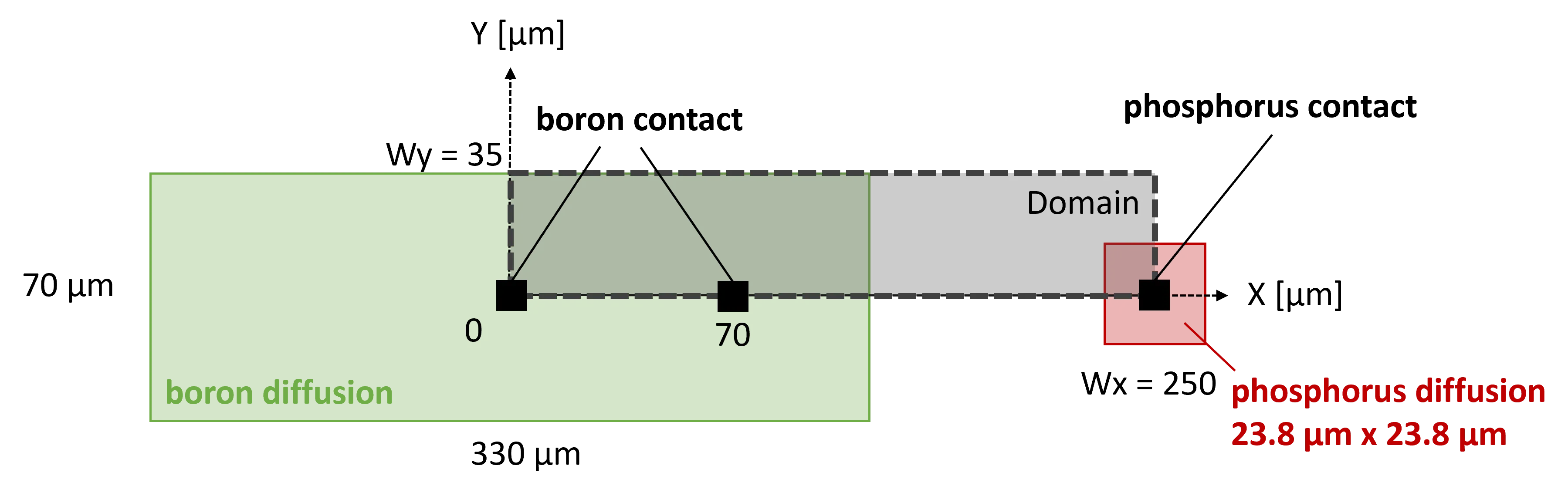
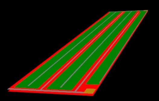
Below image shows the rear side of the ANU IBC example defined via the generic syntax, contained in the 2014 unit cells example.

Simplified syntaxes

front and rear contact unit cell

The scope of this syntax is to define common unit cell solution domains for cell designs having contacts at the front and rear side with a typical H-pattern or full-area metallization. It greatly simplifies geometry definition by not having to figure out and define every position and size of the geometric features. It is an easy starting point into Quokka3, and the recommended syntax for all common non-full-area silicon solar cell simulations.

This syntax supports a ‘busbar enhanced’ unit cell type, where an H-pattern metallization can be set and half of a busbar and half of a finger length is included in the domain. In contrast to the standard unit cells, the ‘busbar enhanced’ one can correctly account for localized shading and recombination of the busbars, and the distributed finger resistance opposed to a lumped series resistance value. If a H-pattern metallization is set both at the front and rear side, bifacial cell designs can thoroughly be modeled.

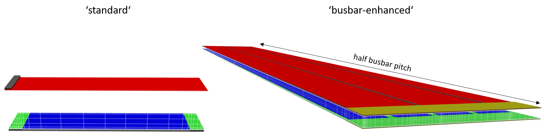
Notably one can set a different contact pitch at the front and rear side, which must otherwise be closely related in common unit-cell simulation, usually being restricted to equal, half or double. Quokka3 finds the least-common multiplier of the two pitches, and this way creates the “true” symmetry element for any pitch combination. However, the user should take care to use sensible numbers, to prevent a very large mesh and simulation time. But there is no limit on practically realizable pitch combinations in Quokka3, as at the far end one can define a full cell with the actual geometry (using the generic syntax).

Conduction types and polarities (n-type or p-type) of all features are ignored, but defined globally via ‘FrontMetalPolarity’ and ‘RearMetalPolarity’, which must be opposite.

front and rear contact full cell

This syntax is similar to the ‘front and rear contact unit cell’ in that it defines a both-sides contacted solar cell with H-patterned or full-area metallization at the front and rear. It differs in that it defines the geometry based on a full-cell view, meaning cell size, busbar and finger numbers, instead of the respective pitches. Most notably, it accounts for edge effects, featuring the optional inclusion of a redundant-line. It further supports a shingle cell layout.

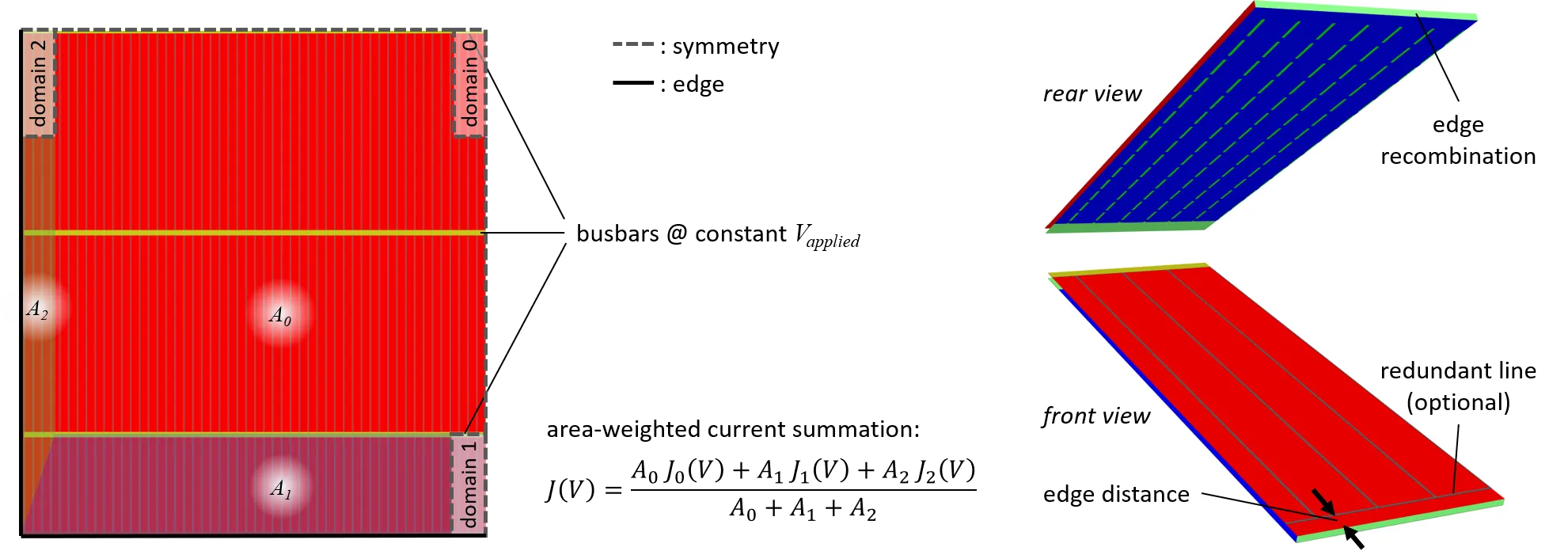
The syntax allows different solution domains to represent the full cell by the ‘FullCellDomainType’ parameter:

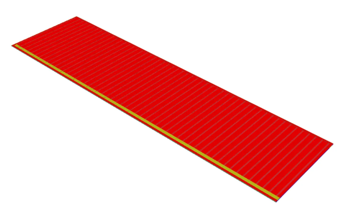
• ‘full’ builds the 3D geometry of the entire cell
• ‘half-symmetry’ and ‘quarter-symmetry’ builds the respective symmetry element only
• ‘multi-domain’, see below

multi-domain approach

The multi-domain approach automatically constructs multiple different solution domains comprising an inner domain and one or two edge domains (for a shingle layout there is only one edge domain). By the sole assumption that the busbars have a constant potential, which is inherit to this simplified syntax anyway, the full-cell characteristics including edge effects can be accurately simulated with a fraction of the computational demand. This in particular enables to accurately simulate full-cell characteristics of more complex cell designs, e.g. featuring dot / dashed rear-contacts, as those would result in prohibitively large meshes for the other full-cell domain types.

An additional benefit is that by comparing the final result from the inner and edge domains the edge losses of the full cell design are directly quantified, whereas the other domain types would require an additional simulation (e.g. a busbar-enhanced unit-cell simulation) as an edge-loss-free reference point.

IBC

The ‘IBC’ syntax defines interdigitated back-contact cells: n-type and p-type skin regions alternate on the rear side, each contacted by a metal finger and optionally separated by a gap; the fingers of each polarity connect to a busbar, and the busbars can carry solder pads. The front side is a single full-area skin. Like the front-and-rear-contact syntaxes, it builds the geometry from pitches and sizes instead of explicit feature positions, and offers solution domains of increasing size and computational cost via the ‘DomainType’ parameter:

• ‘standard’: a simple 2D unit cell across one pair of fingers (the only 2D domain, and therefore the only one within the limits of the free version)
• ‘busbar-enhanced’: covers half of a busbar width and the full finger lengths, to include finger resistance and busbar effects, e.g. for optimizing finger and busbar pitch
• ‘pad-enhanced’: additionally covers half of the solder-pad pitch, to include the busbar transport losses and the solder-pad geometry
• ‘full’: builds the full-cell geometry
• ‘multi-domain’: approximates the full cell including its edges by several subdomains with a minimal mesh and computing time, analogous to the multi-domain approach of the full-cell syntax

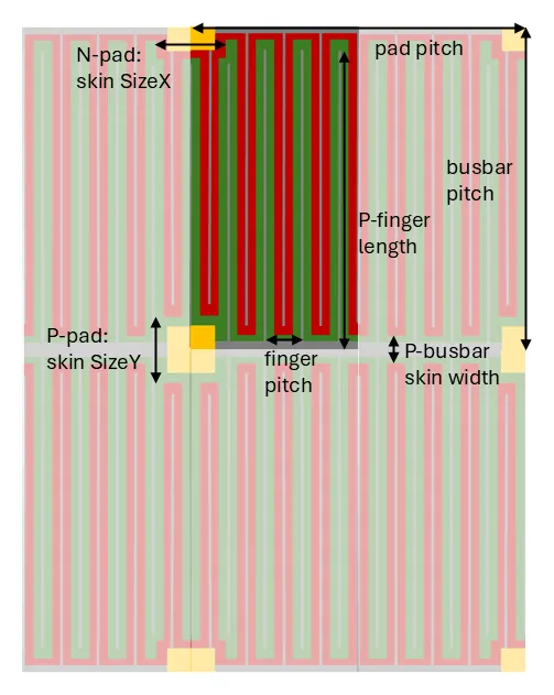
Which geometry parameters apply depends on the domain type: ‘FingerPitch’ for the unit-cell types, ‘BusbarPitch’ for ‘busbar-enhanced’ and ‘pad-enhanced’, and ‘FingersPerPad’ for ‘pad-enhanced’; the full-cell types are instead defined by ‘CellSizeX’, ‘CellSizeY’, ‘FingerNumber’, ‘BusbarNumber’ and ‘OuterFingerPolarity’, with optional solder pads (‘IncludeSolderPads’, ‘PadNumber’, ‘PadEdgeDistance’ or ‘FingersToOuterPad’). ‘CellThickness’ is the cell thickness excluding metallization.

The properties of the rear-side features are set per polarity in the groups ‘PSkin’ / ‘NSkin’ (the skin properties, with the same settings as a generic skin feature), ‘PContact’ / ‘NContact’ (the contacts), ‘PFinger’ / ‘NFinger’ (finger width, length, shading fraction and sheet resistance), ‘PBusbar’ / ‘NBusbar’ (busbar width and skin width, optional busbar contact, shading fraction) and ‘PPad’ / ‘NPad’ (solder pad and pad-skin sizes, contact resistivity between busbar and pad); ‘LocalPContactSkin’ / ‘LocalNContactSkin’ define an additional skin aligned with the finger and busbar contacts. ‘FullFrontSkin’ defines the front side. Further groups cover the gap between the n and p regions (‘GapSkin’, with its width and skin properties), a shunt across the n/p interface (‘NPShunt’, ohmic and / or J02-type), the perimeter and edge skins of the full-cell types, and probes. A 3T device with a front grid can be defined via ‘FrontFinger’ and ‘FrontContact’ (for the ‘standard’ and ‘busbar-enhanced’ domain types) and ‘FrontBusbar’ (‘busbar-enhanced’ only) when the 3T solver settings are enabled.

All parameters are listed in the Settings Reference, and the IBC syntax example walks through the four domain types from the minimal 2D geometry to the full-cell multi-domain model.

Results files

Simulation results are stored in a HDF5 (.h5) file, containing all rendered results. HDF5 is an open-source file format specifically developed to store large datasets of different types into a group-structure. Data can be browsed, read and further processed by many scientific software tools (e.g. Matlab, Mathematica, Python, …). It also contains metadata, e.g. sweep parameter names, units, used version, etc.

After a simulation (local or cloud, from the GUI or the command line), the client additionally writes an Excel (.xlsx) file next to the resultsfile, containing a subset of the results which can be conveniently opened in Excel. For sweeps, only the first 21 sweep points are written automatically; use File → Export → Export Excel resultsfile in the GUI to write the Excel file for any opened resultsfile with the number of sweep points of your choice.

What kind of results are rendered by Quokka3 is dependent on the simulation setup, in particular the solution type (and whether it contains a unique operating point), and the sweep settings. There are 4 different types of results: Scalar, Curves, Maps and Spatial results. They are stored in Groups with the respective name in the HDF5 file, and in separate sheets for the Excel file.

• Scalar: a single numeric value (e.g. Voc). If a sweep is defined, this will be an array of values according to the sweep dimensions. For a two-dimensional sweep (i.e. using GroupA and GroupB sweep parameters), Scalars are stored as 2D arrays in the hdf5 file, which easily allows for e.g. contour plots. In the Excel file the results from a 2D sweep are linearized.
• Curves: curves are rendered only for ‘curve’-solution types. For a sweep, the set of curves for each sweep point is stored in a separate subgroup named ‘/Sweep(ia,ib)/’ in the HDF5 file.
• Maps: The luminescence intensity and some sheet properties of the boundaries are stored as maps. Maps are 2D arrays in the XY plane, and are only stored in the HDF5 file. For a sweep, equivalent subgroups as for Curves are created. Maps may not be stored by default, but can be forced to be stored.
• Spatial: In the HDF5 file spatial data is always stored as 3D arrays, regardless of the dimensions of the solution domain. Note that the order of the dimensions is Z, X, Y. It also contains vectors for the element center and face positions in each coordinate direction. Some spatial results, e.g. current densities, are defined at element face positions rather than centers, and have consequently one more data point in the respective coordinate direction. In the Excel file only 1D spatial data is stored. For a sweep, equivalent subgroups as for Curves are created. Spatial data may not be stored by default, but can be forced to be stored.